The smallest high-order solver that works
In chapter 1 we made the case for high-order (same cost, far less error on smooth flows) and ended on the single idea behind flux reconstruction: discontinuous polynomials inside each element, stitched together by a common interface flux and a correction function. Here we build it. This is the smallest flux-reconstruction solver that actually works: 1D linear advection, a few dozen lines of Python you can read in one sitting.
The result, before any of the code:
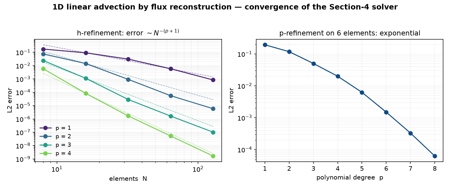
Refine the mesh and the error falls at the design rate; raise the polynomial degree instead and it drops faster than any fixed-order scheme can manage. Here is how a solver this small does that.
The problem
The simplest hyperbolic problem there is,
\[\frac{\partial u}{\partial t} + a\,\frac{\partial u}{\partial x} = 0, \qquad a > 0,\]on a periodic domain. There are no source terms, no nonlinearity and no boundary subtlety to muddy the water, so any error you see is the scheme’s own, the same honesty as the advection experiment in the companion note.
The recipe
Map each element to the reference interval \(\xi \in [-1, 1]\), where \(\mathrm{d}\xi/\mathrm{d}x = 2/\Delta x\). Carry the solution at the \(p+1\) Gauss points, so the in-element solution is a degree-\(p\) polynomial. Then, in reference coordinates, the FR update of the nodal values is
\[\frac{\partial u}{\partial t} = -\frac{2}{\Delta x}\Big[\, \underbrace{\frac{\partial F^{D}}{\partial \xi}}_{\text{element flux}} + \big(f^{*}_{L} - f^{D}_{L}\big)\,g_{L}'(\xi) + \big(f^{*}_{R} - f^{D}_{R}\big)\,g_{R}'(\xi) \,\Big],\]where \(F^{D} = a\,u\) is the element’s discontinuous flux, \(f^{D}_{L,R}\) are that flux extrapolated to the left/right faces, \(f^{*}_{L,R}\) are the common (upwind) interface fluxes, and \(g_{L}', g_{R}'\) are the derivatives of the Radau correction functions, the choice that makes this FR scheme coincide with nodal DG. Advance in time with classical RK4.
Two implementation details are worth flagging because they are the usual places to go wrong:
- The differentiation matrix must be the true derivative of the Lagrange basis, \(D_{ij} = \ell_j'(\xi_i)\). The off-diagonal entry is \(D_{ij} = (w_j/w_i)\,/\,(\xi_i - \xi_j)\) with barycentric weights \(w_j = 1/\prod_{k\neq j}(\xi_j-\xi_k)\), not simply \(1/(\xi_i-\xi_j)\), which is only correct when all the weights are equal (they are not, for Gauss points). The code below uses the correct form. (An earlier draft of this solver had exactly this bug; it is an easy one to make.)
- With Gauss points the solution points are interior, so the face values must be obtained by polynomial extrapolation (
lL,lRbelow), not by reading off an endpoint node.
The code
# 1D linear-advection flux reconstruction (DG / Radau correction) on Gauss points, RK4 in time.
# This is the exact solver behind the convergence figure above: ~p+1 order under mesh
# refinement, and exponential convergence under p-refinement.
import numpy as np
from numpy.polynomial import legendre as L

def diff_matrix(x):
    """Nodal differentiation matrix D[i,j] = l_j'(x_i) for Lagrange basis on nodes x."""
    n = len(x); D = np.zeros((n, n))
    for i in range(n):
        for j in range(n):
            if i != j:
                num = np.prod([x[i] - x[k] for k in range(n) if k not in (i, j)])
                den = np.prod([x[j] - x[k] for k in range(n) if k != j])  # base point x[j]
                D[i, j] = num / den
        D[i, i] = sum(1.0 / (x[i] - x[k]) for k in range(n) if k != i)
    return D

def lagrange_at(x, xq):
    """Values of all Lagrange basis functions l_j at a single point xq."""
    return np.array([np.prod([(xq - x[k]) / (x[j] - x[k]) for k in range(len(x)) if k != j])
                     for j in range(len(x))])

def legendre_deriv(p, xq):
    """P_p'(xq)."""
    c = np.zeros(p + 1); c[p] = 1.0
    return L.legval(xq, L.legder(c))

def fr_advection(p, N, a=1.0, Lx=1.0, tend=1.0, cfl=0.1):
    xi, _ = L.leggauss(p + 1)                      # p+1 Gauss points -> degree-p solution
    D = diff_matrix(xi)
    lL, lR = lagrange_at(xi, -1.0), lagrange_at(xi, 1.0)   # extrapolation to faces
    # Right Radau correction g_R(xi) = 0.5*(P_p + P_{p+1}); here we need its derivative.
    gR = lambda xq: 0.5 * (legendre_deriv(p, xq) + legendre_deriv(p + 1, xq))
    gRp = np.array([gR(x) for x in xi])            # g_R'(xi_i)
    gLp = np.array([-gR(-x) for x in xi])          # g_L'(xi_i), since g_L(xi) = g_R(-xi)
    dx = Lx / N; xc = (np.arange(N) + 0.5) * dx
    X = xc[:, None] + (dx / 2) * xi[None, :]
    u = np.exp(-((X - 0.5) ** 2) / (2 * 0.05 ** 2))        # Gaussian bump
    def rhs(u):
        uL, uR = u @ lL, u @ lR                    # solution at left/right faces, per element
        fL_common = a * np.roll(uR, 1)             # upwind (a>0): left face uses neighbour's right value
        fR_common = a * uR
        dfdxi = (a * u) @ D.T                       # element flux derivative in reference coords
        corr = (fL_common - a * uL)[:, None] * gLp + (fR_common - a * uR)[:, None] * gRp
        return -(2.0 / dx) * (dfdxi + corr)
    dt = cfl * dx / abs(a) / (2 * p + 1); nt = int(np.ceil(tend / dt)); dt = tend / nt
    for _ in range(nt):
        k1 = rhs(u); k2 = rhs(u + 0.5 * dt * k1); k3 = rhs(u + 0.5 * dt * k2); k4 = rhs(u + dt * k3)
        u = u + dt / 6 * (k1 + 2 * k2 + 2 * k3 + k4)
    return X, u
What it does
That is the whole solver. To measure its error, advect the bump for a whole number of periods and compare against the initial condition, the exact answer. The figure at the top of this note is what you get when you refine it two ways.
Hold the degree \(p\) fixed and refine the mesh (left panel): the error falls at the design rate, error \(\sim N^{-(p+1)}\) (the dashed reference slopes), once the mesh resolves the bump. On the finest meshes the observed orders come out clean, about \(4.0\) for \(p=3\) and \(5.0\) for \(p=4\). The low-order curves (\(p = 1, 2\)) are still pre-asymptotic on the coarsest meshes: a narrow feature simply is not resolved by a handful of low-order cells, the same effect the companion note showed.
Hold the mesh fixed and raise \(p\) instead (right panel): on this smooth solution the error drops faster than any algebraic rate, from about \(2\times10^{-1}\) down to \(6\times10^{-5}\) going from \(p = 1\) to \(p = 8\) on just six elements. That is spectral convergence, and it is the whole reason high-order pays off when the flow is smooth and well-resolved.
This solver and the companion note’s animations are the same idea, one dimension apart.