Why high-order? Flux reconstruction, from motivation to method
Most industrial CFD still runs on second-order finite volume, and for good reason. But there is a class of problems, such as turbulence-resolving simulation, aeroacoustics and clean turbomachinery wakes, where second order quietly throws away the very physics you are trying to capture. This note is about why high-order methods exist, where they came from, and what they actually are. Chapter 2 then builds the smallest version that works.
1. Why high-order, and not finite volume?
Here is the whole argument in one experiment. Take a Gaussian and advect it at constant speed around a periodic domain. The exact solution simply translates the bump; after any whole number of periods it returns exactly to where it started, with its shape and amplitude untouched. So whatever the numerical solution has lost is pure scheme error. There is nowhere for it to hide.
Now fix the cost and change only how you spend it. The currency of a simulation is its degrees of freedom (DOF): the number of unknowns you store and march in time. In a solver such as OpenFOAM, this would correspond to the number of cells.
Where do those unknowns live? A finite-volume scheme keeps a single value per cell (the cell average, one constant), so the only way to add detail is to add cells. A high-order method makes a different choice: inside each cell it represents the solution as a sum of basis polynomials,
\[u(x)\;\approx\;\sum_{j=0}^{p} \hat{u}_j\,\phi_j(x),\]a single polynomial of degree \(p\) built from \(p+1\) basis functions \(\phi_j\), each weighted by a coefficient \(\hat{u}_j\). Those coefficients are the unknowns the solver stores and marches in time, and polynomial order is just \(p\), the highest degree the sum can reach. A degree-\(p\) polynomial carries \(p+1\) coefficients in 1D, \((p+1)^2\) on a 2D cell.
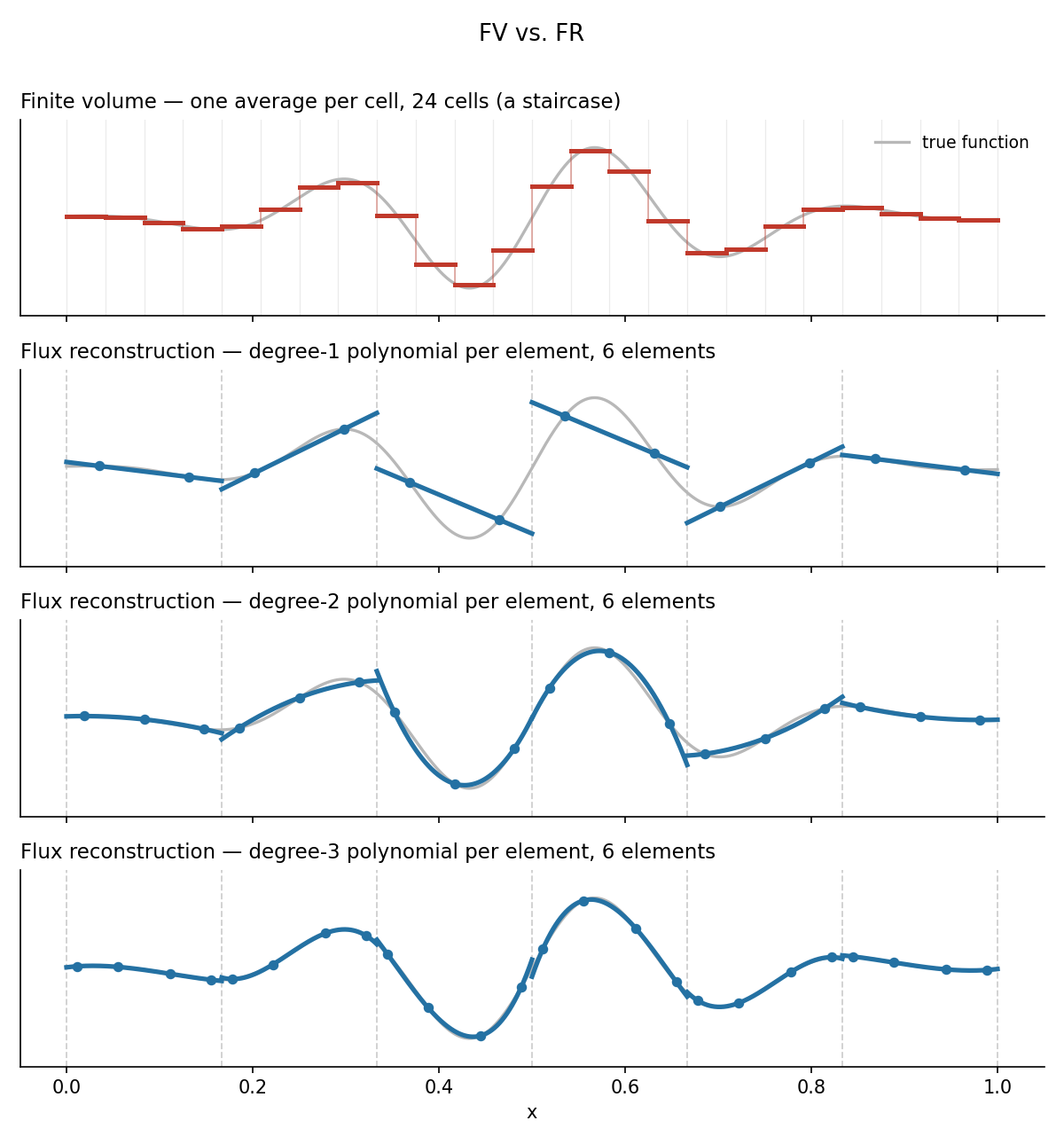
p polynomial inside the cell, the sum of p+1 basis functions (right).Keeping only the single constant \(\hat{u}_0\) is the \(p=0\) case, but that is not how finite volume reaches second order. A production FV scheme also stores one value per cell, then reconstructs a slope from its neighbours’ averages: it buys order across cells rather than storing more coefficients inside them. High-order DG/FR does the opposite, which is what lets you turn the polynomial degree into a knob. So the total DOF is number of cells \(\times\) coefficients per cell, and you can hold that product fixed while shifting the budget from one factor to the other.
Give two runs the same DOF budget and change only how that budget is split between mesh and polynomial order:
- Many small cells, low order: here 4096 unknowns laid out as a \(32\times32\) grid of elements, each carrying a \(p=1\) (linear) polynomial. Resolution comes entirely from having lots of cells; this is essentially the low-order finite-volume picture.
- Few large cells, high order: the same 4096 unknowns as an \(8\times8\) grid of \(p=7\) elements. Now the resolution lives in a high-degree polynomial inside each cell.
Same solver, same cost. Here is the same Gaussian carried twice around the periodic box and back to its starting point:
p = 1 on 32×32 elements.p = 7 on 8×8 elements.The identical Gaussian and the identical 4096 degrees of freedom, advected on a periodic plane and watched over two full laps. Track the peak value printed under each bump: the low-order field loses roughly a third of its height, while the high-order field barely moves.
The low-order field bleeds height on every lap and frays into facets. That amplitude loss is numerical diffusion: energy removed by the discretisation, indistinguishable from a physical viscosity the equation never contained. The faceting and the faint trailing wiggles are dispersion, different wavenumbers travelling at slightly wrong speeds. On an identical budget, the high-order field comes back essentially intact.
The reason high-order wins on smooth flows is accuracy per degree of freedom. A method of order \(q\) (with \(q = p+1\) for a degree-\(p\) polynomial) has error that scales like \(h^{q}\) as the mesh spacing \(h\) shrinks, but you can also buy accuracy by raising the polynomial degree \(p\) instead of refining the mesh. For smooth solutions, \(p\)-refinement converges exponentially, while \(h\)-refinement at fixed low order converges only algebraically. To reach a given error you need far fewer unknowns, which is exactly the regime that matters for LES and DNS, for acoustic propagation over many wavelengths, and for resolving turbomachinery wakes that must survive convection across several blade rows without being smeared into nothing.
There is a reason your production solver is probably still second order: real flows are not smooth. Shocks, sharp gradients and messy industrial meshes are where high-order methods historically broke, and closing that gap is most of this story.
2. A short history of high-order CFD
If high-order is so efficient on smooth flows, why does industry still run mostly second-order finite volume? The answer is robustness, meshing and cost. High-order methods are less forgiving of bad cells, need curved (high-order) meshes to realise their accuracy near walls, and have historically been harder to stabilise around discontinuities. Much of the last two decades of research has been about closing that gap, and a clear European thread runs through it.
That thread is a sequence of EU-funded projects, each picking up where the last left off:
- ADIGMA: Adaptive Higher-Order Variational Methods for Aerodynamic Applications in Industry. An FP6 project (roughly 2006–2009) that brought together European aerospace, DLR and several universities to push discontinuous Galerkin and related variational methods toward aerodynamic problems, with adaptivity as a central theme. Among the partners were the European pioneers of DG for compressible flow, including Francesco Bassi’s group at the University of Bergamo, whose Bassi–Rebay schemes (BR1, BR2) are still a standard way to treat the viscous terms in DG.
- IDIHOM: Industrialisation of High-Order Methods – A Top-Down Approach. The FP7 follow-on (2010–2014), which deliberately started from industrial test cases and worked back toward the methods, rather than the other way around. The name says the intent: make these methods usable, not just publishable.
- TILDA: Towards Industrial LES/DNS in Aeronautics – Paving the Way for Future Accurate CFD. A Horizon 2020 project (roughly 2015–2018) that shifted the target from steady aerodynamics to scale-resolving simulation, where high-order’s advantage is sharpest.
Alongside the projects, two community efforts are worth knowing. The International Workshops on High-Order CFD Methods, first held in 2012 alongside the AIAA Aerospace Sciences Meeting and repeated every couple of years since (the fourth in Crete in 2016, the fifth back at AIAA SciTech in 2018), established a set of shared benchmark cases so that competing high-order methods (DG, flux reconstruction, and high-order finite-difference and finite-volume schemes alike) could be compared on the same problems rather than on each group’s favourite test. And HONOM, the European Workshop on High Order Nonlinear Numerical Methods for Evolutionary PDEs, has long been the meeting point for the more mathematical end of the field.
On the software side, the ideas left the lab some time ago. Codes such as PyFR, Flexi, Nektar++ and the DG/FEM branch of SU2 are open, actively developed, and run high-order schemes on GPUs and large HPC systems today. High-order CFD is no longer a promise; it is a tool you can download.
3. Flux reconstruction, DG and friends: the unifying idea
The conceptual core of this whole family of methods is surprisingly small, and it is worth stating plainly before any equations.
Divide the domain into elements. Inside each element, represent the solution by a polynomial, but do not require those polynomials to match at element boundaries. The numerical solution is allowed to be discontinuous across interfaces. That single choice is what makes the method local, compact and parallel-friendly: each element is largely self-contained.
If your mental model of “finite elements” comes from structural mechanics, this is the key place not to be misled. The classical structural FEM is continuous Galerkin: neighbouring elements share nodes, the field is continuous across the whole mesh, and everything is assembled into one global stiffness matrix, natural for the elliptic problems of elasticity. The CFD methods here are the opposite by design. There are no shared nodes and no global continuity; elements are coupled only weakly, through interface fluxes, exactly the way a finite-volume method couples neighbouring cells. That is the right choice for convection-dominated, hyperbolic problems, where information rides along characteristics and must be upwinded. So DG and FR sit between the two worlds you may already know: finite-element polynomials inside each cell, finite-volume flux coupling between cells.
Of course, a solution that is double-valued at every interface is not a solution to anything yet. Two ingredients fix that:
- A common interface flux \(f^{*}\). At each interface you have two competing values, one from each side. You replace them with a single, shared flux computed by a Riemann solver (for linear advection, simply upwinding). This is the only place neighbouring elements talk to each other, and it is where the physics of wave propagation enters.
- A correction function \(g\). The element’s own (“discontinuous”) flux does not, in general, equal the common flux at the boundary. The correction function is a smooth polynomial that lives on the element and is built to carry the difference between the common flux and the element’s boundary flux back into the interior, in a way that is exact at the boundary and minimally intrusive inside.
Huynh’s original insight, when he introduced flux reconstruction (FR), was that the choice of correction function is a dial. Pick one correction function and FR reproduces nodal discontinuous Galerkin exactly. Pick another and you recover the spectral difference method. Others give you yet more known schemes, and a continuous family of stable schemes in between. One framework, several familiar methods, distinguished only by which correction polynomial you plug in. That is why it is worth learning FR rather than any single scheme: you get the family, not just one member.
That is the idea. The companion note puts it to work: it takes the correction function that recovers DG (the right and left Radau polynomials, on Gauss solution points) and turns it into the smallest 1D solver that actually works, then watches it converge exponentially.